Historical Data Tool
The Historical Data Tool allows you to combine systematic gauged data (continuous observed data) with censored historical flood information in flood frequency estimation and can be accessed via the r-click menu items associated with the Site of Interest.
The historical events are those that exceed a threshold, the Perception Threshold. The methods were developed under the Environment Agency R&D Project SC130009 project, as described in Dixon et. al., 2017, which provides more information on when it may be appropriate to incorporate historical flood data and how to obtain it.
A summary of the maximum likelihood method and how this is different to L-moments used in Single Site analysis, is presented in Parameterisation using the Historical Data and Single Site methods.
The dashboard enables you to estimate the Flood Frequency Curve (FFC) for two cases; the case where you have estimates of flow for your historical events and the case where you only know the number of historical events that exceed the Perception Threshold. You can also review your historical events, systematic AM series and Perception Threshold as a time-series graph.
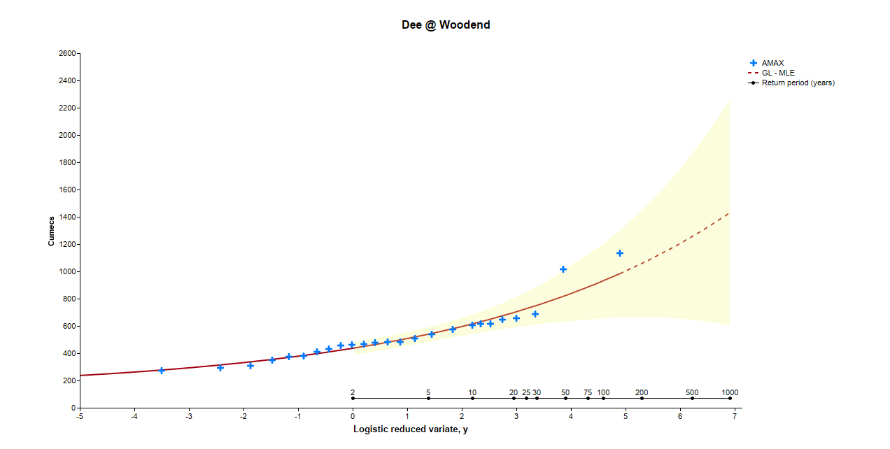
An example of the FFC produced using a pseudo historical record at the Dee at Woodend using Method 1A is presented below.
Importing historical data
Historical data can only be imported from a populated csv file. The format of the csv file must be flow dates in column A and flow values in column B, without any column headers. An example input csv file that can be used as a template is available here. The template provides examples for the range of data formats that can be used:
- It is possible to provide the date in three different forms: as a four digit year value, a month and a year or a complete date with day, month and year. Years must be reported as four digits and days and months must be reported as two digits. Dates must be separated by a “/” symbol and must be numerical. The date can take the following format: XX/XX/XXXX, XX/XXXX, or XXXX, where “X” is numerical.
- Historical flow dates must occur before the start of the systematic record.
- If the date of an event is known but the magnitude of the event is unknown, then provide the year and leave the flow value as blank.
- Flow values must be numerical and have no precision limitations.
The example dataset, in the template, is intended to be used with station 54001 (Severn @ Bewdley) from the NRFA Peak Flow Dataset and is for example purposes only. A Perception Threshold of 550 cumecs and a historical period length of 240 years should be used with this dataset. It is recommended that a text editor, such as Notepad++, is used to modify the input csv file to avoid erroneous formatting being introduced.
Historical Data Tool dashboard
Perception Threshold
The Perception Threshold corresponds to the threshold above which a flood would have been large enough to be noted in historical sources or leave recognisable signs across the catchment. The success of the calculation and the results are very sensitive to changes in the Perception Threshold. Guidelines relating to a suitable choice of Perception Threshold value are outlined in the Environment Agency R&D Project SC130009 reports. The Perception Threshold is constrained to lie between 0 and the lowest historical flow value.
REQMIN
The REQMIN value defines the required precision that the optimisation routine must converge to by defining the required minimum value that the optimised outcome of the routine must not vary by. Increasing the REQMIN value will increase the likelihood that the optimisation routine will successfully converge.
Method 1A – known flow values
This method is applicable when historical peak flow rates are available for all historical events exceeding the Perception Threshold. To fit a flood frequency curve to the gauged (systematic) and historical data, a maximum likelihood method is adopted.
Method 1B- unknown flow values
This method can be applied if you are confident that all floods exceeding the Perception Threshold have been identified but the actual flow rates are unknown. In this application the flow rates for all events in the systematic data are also disregarded and the maximum likelihood considers the total number of events that exceed the Perception Threshold.
Standardise
The Standardise tool applies a standardisation to the results presented in the ‘Flood Frequency Curve’ and the associated table to produce a growth curve and growth factors. The default method is to Standardise by the median of the systematic flow record with an additional option available to standardise by a user defined value.
Method fails to converge -issues with the stability of the solutions
In the event that the maximum likelihood method fails to converge or if WINFAP warns you of stability issues, there are a number of steps that can be taken to increase the chance of successful convergence:
- Re-attempt the analysis with different values for the Perception Threshold. This is often the primary cause of failures in convergence.
- Analyse the position of flows plotted as points on the flood frequency curve. If convergence fails, the flood frequency curve will plot a curve defined by systematic data but will plot flow values for systematic and historical data. If historical flows appear to be anomalous, attempt removing these and re-attempting the analysis.
- Modify the start date of the historical period of time.
- Attempt modifying the REQMIN Value.
Errors associated with importing historical data
If you are experiencing errors when importing your historical data into the historical data tool, you should check the following:
- The date of your latest historical flow should be before the start of the systematic record.
- Invalid date formats such as non-numerical months and invalid date separators. See Importing historical data for more information on valid date formats.
- Formatting errors introduced into the CSV file when formatted and saved using numerical processing software. A text editor is recommended for formatting the input CSV file, such as Notepad++.
Parameterisation using the Historical Data and Single Site methods
When using Historical Data a Maximum Likelihood Method (MLM) is used to estimate the parameters for a Generalised Logistic distribution and fitted to the data. Note that FEH recommends the Generalised Logistic distribution for UK flood data and MLM is the recommended method when extending the Single Site (SS) analysis through the use of historical flood data.
The MLM ‘searches’ for the optimum parameters using a maximum likelihood algorithm. This approach can be time consuming hence initial estimates of the parameters are made from which to start the algorithm. The algorithm then looks for the ‘peaks’ relating to the objective function used to describe how well each parameter set reflects the data. There may be a number of these ‘peaks’ and, whilst efforts are made to ensure that the optimum parameter set is derived, it is possible that a ‘better’ parameter set might exist which is not returned.
In the standard Single Site method the distribution parameters are based on the L-moments of the data in the standard Single Site method. It is not possible to use this method to produce parameter estimates when taking into account 'missing' data.
The distribution parameters derived (just using the systematic data) may therefore be different using the MLM or L-moment methods. If there was an infinitely long times series then both methods would provide the same parameter estimate, however in practise this is rarely the case. Both parameterisations are equally valid.
Estimation of Confidence Intervals
Confidence intervals in the Historical Data Tool are based on estimates of the parameter variances derived from the MLM, which are then combined to determine the variance, hence standard error, of the flows estimated at each return period. The assumption is made that the errors are normally distributed and the 95% confidence limit is subsequently calculated as 1.96 x standard error. Due to the assumption of normality and the fact that the confidence limits are calculated separately for each return period it is possible that these can be very large (for high return periods) and may appear to be inconsistent, for example, where the confidence limits go below the QMED for the 1 in 1000 year return period in the provided example.
The confidence intervals in the Single Site method are derived by bootstrap sampling the data. i.e. numerous examples of ‘equally likely’ AM datasets are produced and the resulting L-moments, parameters and FFC associated with these are calculated. The confidence limits are then derived from the samples. No assumptions about the distribution of the errors are made.
The confidence intervals derived (just using the systematic data) can be quite different from the two methods hence any comparison or interpretation of these should take into account the differences in how they are calculated.